An Introduction to Vectors
One of the workhorses of the R language.
Data Science Altitude for this Article: Sea Level.

Today’s post is about vectors, one of the most common object types in R. It’s designed to be low-level introductory subject matter (thus our ‘Sea Level’ altitude on the mountain) for those that are are at the ‘curio sity’ stage of Data Science: what is it, how does it work, how do I go about getting my feet wet… That sort of thing.
First, let’s start off with some definitions. Depending on your mathematics background, the word ‘vector’ might cause you to wonder if you’re working with something exotic and complicated. Not really. Despite the fact that Merriam-Webster provides no less than seven possible definitions of the term, we’re working here primarily with the first:
…a quantity that has magnitude and direction and that is commonly represented by a directed line segment whose length represents the magnitude and whose orientation in space represents the direction.
The word ‘Vector’ originates from Latin, meaning ‘to convey’ or ‘to carry’. So what are we conveying here? Let’s break down the term into something we can compare and contrast with past experience with spreadsheets, mathematics, or concepts found in everyday life.
This takes us to the first function used by many who have worked with R: c(), the combining of values into a resulting vector.
Don’t have an environment where you can run this code? No worries, that’s the subject of the next post, where we will go into the ‘user experience’ of installing the free version of R and R Studio on your home PC or laptop.
Our First c() Command to Create a Vector:
# Define a vector named gasPerGallon with four values.
gasPerGallon <- c(2.75, 2.55, 2.88, 3.58)
# Print out the values to the console
gasPerGallon
## [1] 2.75 2.55 2.88 3.58
You might be wondering what this has to do with our prior definition of a vector. We see magnitudes, but what does direction have to do with this? We’re missing something here.
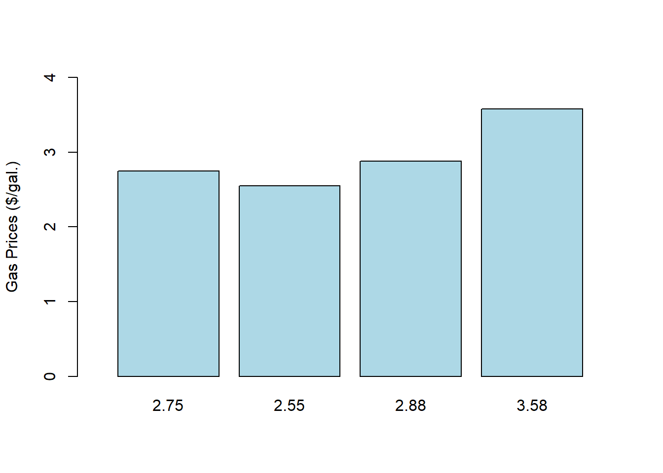
The answer is that these values shouldn’t be considered in a vacuum. These are observations of a single characteristic: gas prices. But they could be measurements starting at a particular point in time for a single gas station over several months. They could be gas prices on the same date in different locations across the world. You get the idea. To understand what the numbers represent, we need more context.
Vectors Imply a Shared Data Context
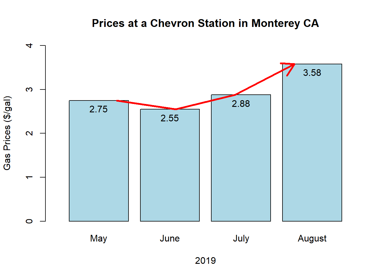
In short, the difference between a vector and just a collection of numbers to be grouped together is their shared context. Let’s look at this information a little differently, from the perspective that these are from the same gas station across a time interval.
Now we have magnitude and direction, in context - a time frame of observations for a single gas station of one characteristic, gasoline prices.
One Data Context for a Vector = Only One Data Type Returned
The following code involves the use of the sprintf() string formatting call, likely very familiar to those of you with a C programming background. Also used here is the class() call, which communicates what type of object and type you have.
It wouldn’t make much sense to modify a vector like what we’ll do with vector b below. R will let you, but you might not like the result:
vector_b <- c(1.2, 2.3, 3.4, 4.5)
vector_b
## [1] 1.2 2.3 3.4 4.5
sprintf("All the values of b are %s.", class(vector_b))
## [1] "All the values of b are numeric."
# Introduce a character string as the fifth element of a numeric vector
vector_b[5] <- "5.6"
sprintf("All the values of b are now %s:", class(vector_b))
## [1] "All the values of b are now character:"
vector_b
## [1] "1.2" "2.3" "3.4" "4.5" "5.6"
What we’ve done by introducing a character value as the fifth value of the vector is to invoke R’s need to keep singular a vector’s type. It does that by coercion, an under-the-covers process to determine what’s the most consistent treatment for all data values being considered.
It’s a lot easier to change the number 5.3 into “5.3” than changing the word “help” into a number, for example. The first way involves a pretty consistent method, the second doesn’t. So don’t mix data types in vectors, otherwise R will do what it has to do to remain internally consistent. From the R Documentation:
Vectors must have their values all of the same mode. Thus any given vector must be unambiguously either logical, numeric, complex, character or raw… numeric mode is actually an amalgam of two distinct modes, namely integer and double precision…
Explicit Setting Of Class, Where Permitted
Meaning, you can force a vector to be of integer class - for example - using an explicit as.integer() coercion call. But be forewarned, square pegs can’t always be put into round holes; vector_f doesn’t care to have text data coerced into an integer. It can, however, figure out how to convert the text version of a number:
vector_d <- c(1, 2, 3, 4)
sprintf("All the values of vector_d are %s.", class(vector_d))
## [1] "All the values of vector_d are numeric."
vector_d
## [1] 1 2 3 4

vector_d <- as.integer(c(1, 2, 3, 4))
vector_d
## [1] 1 2 3 4
sprintf("All the values of vector_d are %s.", class(vector_d))
## [1] "All the values of vector_d are integer."

vector_f <- as.integer(c(1, 2, 3, "bad idea"))
## Warning: NAs introduced by coercion
vector_f
## [1]  1  2  3 NA

vector_f <- as.integer(c(1, 2, 3, "5.2"))
vector_f
## [1] 1 2 3 5
Python Has Similar Constructs to R Vectors
And we’d be remiss not to do a brief shoutout to Python’s similar construct, the Series. It is also of a singular data type. Though Python’s primary data objects are lists and dictionaries - a discussion for another day - methods in the numpy and pandas packages provide indispensable support for vectorized concepts:
import numpy as np
import pandas as pd
pythonGasArray = np.array([2.75, 2.55, 2.88, 3.58])
print(pythonGasArray)
## [2.75 2.55 2.88 3.58]
pythonGasSeries = pd.Series(pythonGasArray)
# Converted Pandas series from a numpy array
print(pythonGasSeries)
## 0    2.75
## 1    2.55
## 2    2.88
## 3    3.58
## dtype: float64
print("The average gas price in the 4-month period is {0}".format(pythonGasSeries.mean()))
## The average gas price in the 4-month period is 2.94
Gaps in your Vector’s Data? No Problem.
Suppose you’ve written a program that loops through a dataset and you’re saving off results for each pass through the loop in a vector. If you’ve made a mistake in your code, you may have some ‘holes’ in your vector values where data is not available (NA).
You could just as easily have read in a dataset with some missing values.
vector_e <- c(1.2, 2.3, 3.4, 4.5)
vector_e
## [1] 1.2 2.3 3.4 4.5
# Set the eighth element of the vector, effectively leaving elements 5, 6, and 7 empty.
vector_e[8] <- 5.6
vector_e
## [1] 1.2 2.3 3.4 4.5  NA  NA  NA 5.6
Luckily, there are several ways to identify and remove those. Next up: the which() and is.na() commands along with the negation (!) operator.
First, the is.na() call returns a vector of TRUEs and FALSEs noting whether data is missing (not available) for each of the elements in the vector. TRUEs and FALSEs are known as boolean values, only able to take on those two values, and stored as a zero or a one.
The negation operation (!) can flip those values, showing which data is good instead of bad.
A call to which() returns the position of the elements that satisfy a test.
# Which data is bad?
is.na(vector_e)
## [1] FALSE FALSE FALSE FALSE  TRUE  TRUE  TRUE FALSE
# Which data is good?
!is.na(vector_e)
## [1]  TRUE  TRUE  TRUE  TRUE FALSE FALSE FALSE  TRUE
# Which elements of the vector can the bad data be found in?
which(is.na(vector_e))
## [1] 5 6 7
# Set vector_f to only the non-missing values of vector_e
# You could also overwrite vector_e with its own subset.
vector_f <- vector_e[!is.na(vector_e)]
vector_f
## [1] 1.2 2.3 3.4 4.5 5.6
Further Information on the Subject:
This post just scratches the surface of vectors, and of beginning R syntax in general. For something a little more in-depth, you can consult some of the following:
A good Stack Overflow post on the topic of type coercion. In later posts, we’ll cover why Stack Overflow is another must-bookmark resource.
The topic as presented on r-tutor.com.
A good book on the functionality of base R, from the ground up. From vectors to modeling and then some: The R Book, by Michael J. Crawley.
The documentation for the numpy and pandas Python packages are a must-bookmark part of any data scientist’s browser and are all part of the SciPy product ecosystem.