Probabilistic Topic Models and Latent Dirichlet Allocation: Part 4
From Data Formatting to Model Formation and Object Characteristics. All this effort is about to pay off...
Data Science Altitude for This Article: Camp Two.
Previously, we created a DocumentTermMatrix for the express purpose of its fitting in nicely with our upcoming LDA model formation. Here, we’ll discuss LDA in a bit of detail and dive into our findings. But first, a brief refresher on the format and content of the DT matrix. The word count for the first ten stemmed words out of the first eight documents and their aggregation for documents 9-85 are seen below:
# If you're curious as to how the table below was built:
data = as.matrix(dtMatrix[1:8,1:10])
data2 = as.vector(colSums(as.matrix(dtMatrix[-(1:8),1:10])))
data3 = as.vector(colSums(as.matrix(dtMatrix[,1:10])))
knitr::kable(rbind(data, 'Rows 9-85' = data2, Totals = data3), format = "markdown", row.names = TRUE)| abl | absurd | accid | accord | acknowledg | act | actuat | add | addit | address | |
|---|---|---|---|---|---|---|---|---|---|---|
| 1 | 1 | 1 | 1 | 1 | 1 | 1 | 1 | 1 | 1 | 1 |
| 2 | 0 | 0 | 0 | 0 | 0 | 0 | 0 | 0 | 0 | 0 |
| 3 | 2 | 0 | 0 | 1 | 2 | 1 | 1 | 1 | 1 | 0 |
| 4 | 1 | 0 | 0 | 1 | 0 | 1 | 0 | 0 | 0 | 1 |
| 5 | 0 | 0 | 0 | 0 | 0 | 1 | 0 | 0 | 0 | 0 |
| 6 | 0 | 0 | 0 | 1 | 0 | 0 | 0 | 0 | 0 | 0 |
| 7 | 2 | 0 | 0 | 0 | 0 | 1 | 0 | 0 | 2 | 0 |
| 8 | 2 | 0 | 0 | 0 | 0 | 1 | 0 | 0 | 0 | 0 |
| Rows 9-85 | 66 | 19 | 1 | 67 | 21 | 134 | 9 | 32 | 57 | 20 |
| Totals | 74 | 20 | 2 | 71 | 24 | 140 | 11 | 34 | 61 | 22 |
Transitioning to our LDA Model
To see how this data layout makes sense for LDA, let’s first dip our toes into the mathematics a bit. We noted in our first post the 2003 work of Blei, Ng, and Jordan in the Journal of Machine Learning Research, so let’s try to get a handle on the most notable of the parameters in play at a high level.
You don’t have to understand all the inner workings of an internal-combustion engine in order to be able to drive a car, but you’d be remiss if you didn’t understand the fundamentals of what keeps it in working order. The same applies here. Let’s just get a basic feel for some of the moving parts. I’m learning as I go along here too…
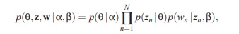
There are five parameters of note in equation 2 at the bottom of page 996 of their paper, denoting the joint distribution of topics: p(θ, z,w|α,β). From there, it’s decomposed into being the product of several conditional probabilities. There are six if you count N, the number of words in all documents.
theta: parameters of the posterior topic distribution for each document, stored as a matrix of documents and topics. You’ll see it as gamma in the model object. I can also show you how to derive this yourself.
z: it’s the topic number assignment for each word in each document, as ordered by the words in w.
w: this is essentially the document term matrix - the count of words in all documents
Given the following conditions:
alpha: a single numeric parameter of the Dirichlet distribution for topics over documents. We’ll find some documentation later that will cover its importance.
beta: logarithmized parameters of the word distribution for each topic. It’s a matrix of topics and stemmed words. We’ll show how to derive this as well.
LDA Model Fitting Rationale
To look at those five parameters more closely, let’s build an LDA model and see where they appear. I’ve done so for a four-topic model, and have made what I think is a pretty safe assumption in saying that there are at least that many throughout the 85 papers. The code below sets it up. The documentation for the LDA call itself tips our hand as to the rationale for our work earlier to create a DocumentTermMatrix. It’s needed as the function’s principal object.
The code is almost identical between the creation of 3-topic and 4-topic objects; the only difference is the setting of k for the number of topics. If you’d like to see examples of what the output looks like when you progress from three topics to four, there’s more detail in the word doc found in my GitHub repo. It’s my original class paper on the subject. I’ll stick with a 4-topic evaluation here, otherwise, we’d have to go over a lot of information twice and we might as well focus on the final conclusions…
burnin <- 1000
iter <- 1000
thin <- 100
nstart <- 10
seed <- rep(list(1),nstart)
best <- TRUE

#LDA() takes several minutes with the given control parms.
ldaOut4 <- LDA(dtMatrix, k=4, method="Gibbs",
               control=list(nstart=nstart, seed = seed, best=best,
                            burnin = burnin, iter = iter))
The control parameters govern the behavior of the LDA call. We’ll get to them shortly. But first, let’s talk about Gibbs Sampling. It’s not the default fitting method. VEM (variational expectation-maximization) is, as explained in Appendix A of the Blei, Ng, and Jordan paper.
The abstract for the topicmodels R package that we added to the environment notes why Gibbs might be preferred over the default VEM model. On page 16:
Due to memory requirements package topicmodels will for standard hardware only work for reasonably large corpora with numbers of topics in the hundreds. Gibbs sampling needs less memory than using the VEM algorithm and might therefore be able to fit models when the VEM algorithm fails due to high memory demands.
So it’s more efficient in its processing. That’s nice, but what’s the difference otherwise? To summarize from the wiki page on Gibbs Sampling:
Gibbs sampling is applicable when the joint distribution is not known explicitly or is difficult to sample from directly, but the conditional distribution of each variable is known and is easy (or at least, easier) to sample from.
That lines up with the following statement in Blei, Ng, and Jordan (Introduction, pg. 995):
Conditionally, the joint distribution of the random variables is simple and factored while marginally over the latent parameter, the joint distribution can be quite complex.
So far, so good.
LDA Control Hyperparameters
Now, about those control parameters… Whenever you have processes that internally make multiple passes to optimize their solutions, control parameters are usually where you find them. LDA is no different.
Taking a set of parameters forced to be of type list, notice iter. It controls the maximum number of iterations in which the method can be refined. nstart is also important. Depending on the value provided, using it is an attempt to ensure that methods that sometimes converge to ‘local’ best solutions get a chance to find ‘global’ best solutions. However, we’ve also hard-seeded the random number generator.
If you’re looking to have reproducible results, you have to set a seed for when you use methods that rely on random starting points. Just don’t cherry-pick to find one that best fits your argument.
The best parameter tells LDA to keep ‘only the model with the maximum (posterior) likelihood’. I’m guessing that’s stashed in the loglikelihood element. We’ll prove that correct shortly.
As with many methods that employ hyperparameters, some rules of thumb are:
- Read the documentation for the types of model(s) you intend to employ, and
- Design your model selection process so that multiple sets of hyperparameters are evaluated. Have a few passes using the VEM method. Try a longer and shorter iteration span, and so forth. And for goodness sake, set up a storage structure to record your results and score for each of your trials so you can get back to the settings that provide you the best model scoring and effectivity. In this case, it looks like loglikelihood…
Even though I admit I’ve violated #2 here for purposes of illustration, those are good rules to live by.
LDA Object Structure
Here’s the structure of the resulting LDA object (ldaOut4):
str(ldaOut4)
## Formal class 'LDA_Gibbs' [package "topicmodels"] with 16 slots
##   ..@ seedwords      : NULL
##   ..@ z              : int [1:87290] 2 3 4 3 3 1 2 2 2 1 ...
##   ..@ alpha          : num 12.5
##   ..@ call           : language LDA(x = dtMatrix, k = 4, method = "Gibbs", control = list(nstart = nstart,      seed = seed, best = best, burnin | __truncated__
##   ..@ Dim            : int [1:2] 85 4890
##   ..@ control        :Formal class 'LDA_Gibbscontrol' [package "topicmodels"] with 14 slots
##   .. .. ..@ delta        : num 0.1
##   .. .. ..@ iter         : int 2000
##   .. .. ..@ thin         : int 1000
##   .. .. ..@ burnin       : int 1000
##   .. .. ..@ initialize   : chr "random"
##   .. .. ..@ alpha        : num 12.5
##   .. .. ..@ seed         : int [1:10] 1 1 1 1 1 1 1 1 1 1
##   .. .. ..@ verbose      : int 0
##   .. .. ..@ prefix       : chr "C:\\Users\\caust\\AppData\\Local\\Temp\\Rtmp4kczGb\\file3a84663224cc"
##   .. .. ..@ save         : int 0
##   .. .. ..@ nstart       : int 10
##   .. .. ..@ best         : logi TRUE
##   .. .. ..@ keep         : int 0
##   .. .. ..@ estimate.beta: logi TRUE
##   ..@ k              : int 4
##   ..@ terms          : chr [1:4890] "abl" "absurd" "accid" "accord" ...
##   ..@ documents      : chr [1:85] "1" "2" "3" "4" ...
##   ..@ beta           : num [1:4, 1:4890] -12.18 -6.67 -12.42 -6.1 -12.18 ...
##   ..@ gamma          : num [1:85, 1:4] 0.181 0.156 0.209 0.142 0.159 ...
##   ..@ wordassignments:List of 5
##   .. ..$ i   : int [1:45328] 1 1 1 1 1 1 1 1 1 1 ...
##   .. ..$ j   : int [1:45328] 1 2 3 4 5 6 7 8 9 10 ...
##   .. ..$ v   : num [1:45328] 4 3 4 2 3 1 2 2 2 1 ...
##   .. ..$ nrow: int 85
##   .. ..$ ncol: int 4890
##   .. ..- attr(*, "class")= chr "simple_triplet_matrix"
##   ..@ loglikelihood  : num -572166
##   ..@ iter           : int 2000
##   ..@ logLiks        : num(0)
##   ..@ n              : int 87290
Before we get to parsing out our five primary parameters, I’ve added two here at the start that you’ll see as we move forward. You can also find more info on the variable definitions on the LDA wiki page.
n: This is the total stemmed wordcount throughout all of the documents. There are 87290 once we finished with the cleaning. That’s also the sum total of our word counts by document in the DocumentTermMatrix.
loglikelihood: For model scoring and determining what the ‘best’ result of each iteration is that we noted in the control parameters… From the package docs on page 4:
For maximum likelihood (ML) estimation of the LDA model the log-likelihood of the data, i.e., the sum over the log-likelihoods of all documents, is maximized with respect to the model parameters α and β.
sum(dtMatrix)
## [1] 87290
logLik(ldaOut4)
## 'log Lik.' -572166.1 (df=19560)theta: Again, you’ll find this in the gamma component of the LDA object. With 85 rows and 4 columns, each row corresponds to a document and each column to a topic. This parameter is not log-scaled as beta is. These are the probabilities that a paper belongs to a specific topic! More on that in the next post.
Recreation - less the str() wrapper to show structure - is as follows:
str(posterior(ldaOut4)$topics)
##  num [1:85, 1:4] 0.181 0.156 0.209 0.142 0.159 ...
##  - attr(*, "dimnames")=List of 2
##   ..$ : chr [1:85] "1" "2" "3" "4" ...
## ..$ : chr [1:4] "1" "2" "3" "4"z: Each word in each document gets a topic assigned to it. That would make this list element of length 87290, as n is calculated above.
Let’s consider parameters z and w together. As specified on page 10 of the package docs:
In additional slots the objects contain the assignment of terms to the most likely topic and the log-likelihood which is… log p(w|z) for LDA using Gibbs sampling…
w: Here’s the structure of our DocumentTermMatrix.
str(dtMatrix)
## List of 6
##  $ i       : int [1:45328] 1 1 1 1 1 1 1 1 1 1 ...
##  $ j       : int [1:45328] 1 2 3 4 5 6 7 8 9 10 ...
##  $ v       : num [1:45328] 1 1 1 1 1 1 1 1 1 1 ...
##  $ nrow    : int 85
##  $ ncol    : int 4890
##  $ dimnames:List of 2
##   ..$ Docs : chr [1:85] "1" "2" "3" "4" ...
##   ..$ Terms: chr [1:4890] "abl" "absurd" "accid" "accord" ...
##  - attr(*, "class")= chr [1:2] "DocumentTermMatrix" "simple_triplet_matrix"
## - attr(*, "weighting")= chr [1:2] "term frequency" "tf"alpha: Yet one more setting you can vary in the control parameters to find the best model in terms of log likelihood… This is a scaling factor noted in the package docs on page 8, and affects the distribution of documents to topics. The default for alpha is given as the ratio 50/k, and since we’ve chosen k = 4 topics, our default alpha is 12.5. You’ll also find on page 13-14 that:
…the lower alpha the higher is the percentage of documents which are assigned to one single topic with a high probability.
beta: Notice that the dimensions of the matrix are 4 rows by 4890 columns. So each row is a topic and each column is a unique stemmed word. You can recreate it - again, less the str wrapper** by the following code. Note that the LDA object class docs say that beta should be on a log scale.
str(log(posterior(ldaOut4)$terms))
##  num [1:4, 1:4890] -12.18 -6.67 -12.42 -6.1 -12.18 ...
##  - attr(*, "dimnames")=List of 2
##   ..$ : chr [1:4] "1" "2" "3" "4"
##   ..$ : chr [1:4890] "abl" "absurd" "accid" "accord" ...
Looking Ahead
The following post will be the last in this series, taking a look at words most common to the topic count (4) we specified and the papers that the LDA model finds most probably comprise them. We’ll use the topics() and terms() methods that provide us the most likely terms for each topic or the most likely topics for each document.
We’ll also be using the LDAVis package to visualize the results!
Further Information on the Subject:
Here’s a superbly composed YouTube video by Andrius Knispelis on some uses of LDA he encountered while working at issuu, the Danish startup he joined in 2011.
And about as complete a dissertation as you can get on the matter of text mining: Text Mining with R. Julia Silge and David Robinson give some concrete examples and a thorough explanation of them.
And if you feel I’ve messed something up here and need to revise, feel free to comment below!