Probabilistic Topic Models and Latent Dirichlet Allocation: Part 3
From Data Cleaning to Data Formatting: Finding a statue within a block of marble.
Data Science Altitude for This Article: Camp Two.
Previously, we removed a bunch of metadata from The Federalist Papers that was introduced from its being hosted by the team at The Gutenberg Project. After that, we took out much of the intra-document metadata that was explanatory in nature to each of the 85 essays.
Now, our goal is to polish off the metadata removal and transition the original unstructured data into object types that are more conducive to numerical analysis.
Breaking Up the Text Vector Upon Document Boundaries
To move this process along, we need to take our long text vector and carve it up into documents delimited by chapter headings (FEDERALIST NO. XX). The code block below is an intermediate step and you’ll see why it’s necessary when we get to the code block following this one.
workList = list(NULL)
for(i in 1:length(chap.positions.v)) {
  if(i < length(chap.positions.v)) {
    workList[[i]] <- text.v[(chap.positions.v[i]+1):(chap.positions.v[i + 1]-1)]
  }
  else {
    workList[[i]] <- text.v[(chap.positions.v[i]+1):length(text.v)]
  }
}

# An example of list element 2 (for Federalist No. 2) with blank lines suppressed.
head(workList[[2]] [workList[[2]] != ""])
## [1] "Concerning Dangers from Foreign Force and Influence"
## [2] "JAY"
## [3] "WHEN the people of America reflect that they are now called upon"
## [4] "to decide a question, which, in its consequences, must prove one of"
## [5] "the most important that ever engaged their attention, the propriety"
## [6] "of their taking a very comprehensive, as well as a very serious,"
A few comments on the code:
Initializing the worklist as a null list makes it possible for the loop to correctly stash elements as type ‘list’.
The loop goes from 1 to the length of the chap.positions.v vector. There are 85 chapters, so a vector length of 85 thus 85 passes through the loop since we cleaned out the duplicate Federalist No. 70 in the prior post…
Each of these list elements starts at the line AFTER the current chapter delimiter and ends at the line BEFORE the next chapter delimiter. We should not see the FEDERALIST delimiter in any of the list elements.
We have a boundary condition to code for in order to process the last chapter correctly. There is no next chapter delimiter, so we have to use the length of the document as the final end-boundary.
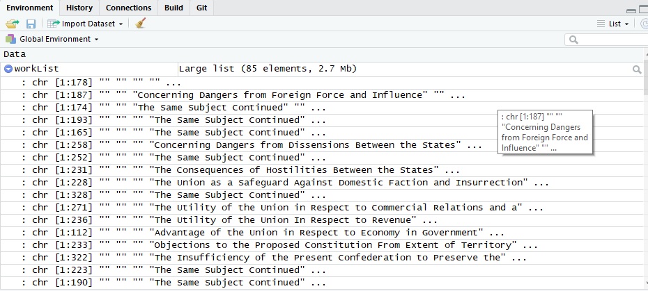
Where we arrive after this section of code is with a list object that has 85 different list elements. Each of these list elements contains a character vector which in turn has one element for each line, including the blank lines. That structure will become more clear in the screenshot from the RStudio environment.
And here’s what the list looks like in the RStudio environment viewer. Note that our chapter delimiters are nowhere to be seen, and we now have 85 list entries, one for each essay. So far, so good…
From List to DataFrame
Even though we’ve got our 85 papers in one of 85 different list elements, that was just an intermediate step to help us build a dataframe. The dataframe - either here in base R or as implemented in the pandas package in Python - is one of the most heavily-used objects in Data Science.
The ins and outs of constructing dataframes are a post for another day, but think of it as a spreadsheet where each column is a vector. We defined vectors in one of our earlier posts: A grouping of data with a shared context and with a singular storage type. A pretty picture to illustrate a dataframe’s similarity to a spreadsheet follows this code block:
workList2 = data.frame(Text = rep(NA, length(chap.positions.v)))
for(i in 1:length(chap.positions.v)) {
  workList2[i,1] = as.vector(paste(unlist(workList[[i]]), collapse = " ")) # row i column 1
}
workList2$Paper = sprintf("Fed %d", 1:85)
workList2$Author = c("Hamiltion", rep("Jay",4), rep("Hamilton",4), "Madison", rep("Hamilton",3),
                     "Madison", rep("Hamilton",3), rep("Madison",3), rep("Hamilton",16),
                     rep("Madison",12), rep("Disputed",10), rep("Hamilton",3), rep("Disputed",2),
                     "Jay", rep("Hamilton",21))
workList2$Label = sprintf("%s:%s",workList2$Paper, workList2$Author)
Some more code commenetary:
- First off, we’ve initialized our ‘spreadsheet’ dataframe with a column called ‘Text’ and set it to 85 uninitialized entries (again, the length of the chap.positions.v vector).
- Now we’re going to loop through each of our list elements in workList1 and make it a ‘cell’ in our worklist2 ‘spreadsheet’. At the end of the loop, we have an 85-row, 1-column dataframe where the column name is ‘Text’.
- The unlist() and paste() function combination flattens the list entry for the text of the paper and makes one big long string of it.
- Then, we’re going to add a column called ‘Paper’. It’s nothing more than a short identifier to the Federalist paper number. Now we have an 85-row, 2-column dataframe.
The ‘Author’ column data is manually added. It might be handy in our analysis to see if some of our topics concentrate with certain authors… The rep function is just a repeat function for when we have the same author consecutively.
A historical note: Some of the authorships are disputed and several analytical efforts (one here) have been undertaken to suggest the identity of the original author(s).
The ‘Label’ column is just the concatenation of paper and author. We are done constructing our dataframe, now at 85 rows, 4 columns.
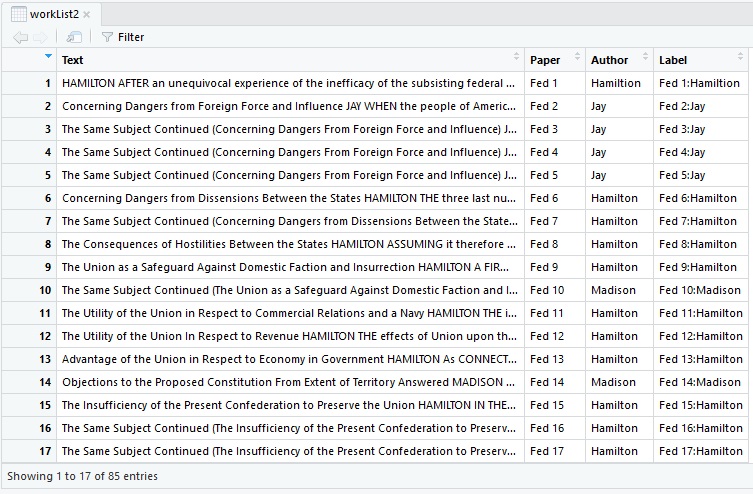
The extra spacing between words still exists, as does the author’s name that we left in here on purpose. Both of those problems will be solved in the next section.
Here’s an example of the text from the beginning of Federalist No. 2, accessing a substring of the second row of the workList2 dataframe’s Text column. Coming up: a heavy dose of the functions and object types introduced in the text mining package tm.
str_sub(workList2$Text[2], start=1, end=98)
## [1] "  Concerning Dangers from Foreign Force and Influence   JAY     WHEN the people of America reflect"
Creation of a Text Corpus
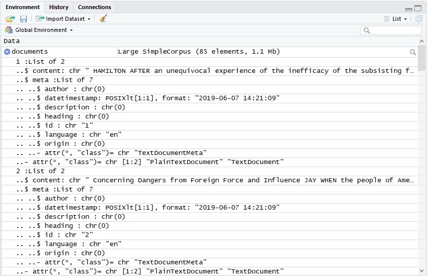
What exactly is a corpus in the context of text mining? Simply put, it’s a list of document text that has specific names and purposes for each of the list elements. Building one from the Text column of our workList2 dataframe…
documents <- Corpus(VectorSource(workList2$Text))…we get a structure that looks something like this - a list of 85 elements, one for each document. Within each of those, a sub-list of two elements, ‘content’ and ‘meta’. ‘meta’ is itself a list as well, providing metadata about the creation and characteristics of that document.
Several different flavors of corpus exist, and there are some subtle and not so subtle differences between them.
Text Corpus Content Refinement
Now that the text is transformed into a corpus, we can use the tm_map() function to perform operations on the ‘content’ element in each of our 85 documents in the corpus. The call takes a corpus and either a function found in getTransformations() or a custom transformation you create with content_transfomer(), as seen below converting all of the content to lowercase.
getTransformations()
## [1] "removeNumbers"     "removePunctuation" "removeWords"
## [4] "stemDocument"      "stripWhitespace"

documents <- tm_map(documents, removePunctuation)
documents <- tm_map(documents,content_transformer(tolower))
documents <- tm_map(documents, removeNumbers)
You may remember that we left the authors’ names in the document along with their common nom-de-plume, Publius. Now it’s time to remove them to further illustrate the concept of ‘stopwords’ as it applies to the removing of common words from a corpus. No sense using ‘a’, ‘an’, ‘the’, ‘is’, or any other common word to determine thematic intent. All are removed from the ‘content’ element of the corpus for each document.
And notice that you have to supply a language to specify the correct set of stopwords. Makes sense… Also notice that all of the extra pesky whitespace will be removed as well.
documents <- tm_map(documents, removeWords,
             c(stopwords("english"), "jay", "hamilton", "madison", "publius"))
documents <- tm_map(documents, stripWhitespace)
Now, time for stemming. As discussed in an earlier post, this is the process of taking words that have a common root origin and replacing them with that root. For example, ‘vibrate’, ‘vibrating’ and ‘vibration’ should all be considered as three instances of the root ‘vibrat’. All three would be replaced in the corpus with the root word.
Notice that I have one of the stemming commands commented out. I’ve tried out both the default stemmer function stemDocument from the tm package and the wordStem function from the SnowballC package. One gives a better topic separation than the other, which I can’t illustrate now because it would mean jumping ahead to our final post. But suffice it to say for now that the more differentiated that topics are from each other, the better.
So, something to file away for our last post, in a section on how to improve upon the findings: More research is needed on the stemming differences between package offerings. I don’t want to dive down a rabbit hole here and ‘let the perfect be the enemy of the good’, as they say…
# Stem the document for topic modeling
#documents <- tm_map(documents, wordStem)    # wordStem as part of the SnowballC package
documents <- tm_map(documents, stemDocument) # stemDocument as part of the tm package

# An excerpt of cleaned and stemmed text from Federalist No. 13
str_sub(documents[[13]]$content, start=1, end = 60)
## [1] "advantag union respect economi govern connect subject revenu"
Creation of a DocumentTermMatrix
Time for the last section of our post. The creation of a DocumentTermMatrix is the jumping-off point for our upcoming statistical analysis. Taking a corpus as its primary parameter, it returns a count of stemmed words for each document as seen below in the example. It also plays very nicely with the needed mathematics of Latent Dirichlet Allocation, as we’ll see in the upcoming post.
dtMatrix <- DocumentTermMatrix(documents)

# dtMatrix excerpt and word frequencies
inspect(dtMatrix)
## <<DocumentTermMatrix (documents: 85, terms: 4890)>>
## Non-/sparse entries: 45328/370322
## Sparsity           : 89%
## Maximal term length: 18
## Weighting          : term frequency (tf)
## Sample             :
##     Terms
## Docs can constitut govern may nation one peopl power state will
##   10   4         3     17  16      4   8     4     2     5   30
##   22   6         6     14  20     14  10     9    18    33   11
##   38   9        16     21   9      1  13     5    24    20   12
##   41   9        20     13  23     14   8     8    40    16   25
##   43   9        24     28  25      2  13     2    11    70   20
##   63  14         8     16  18      9   9    41     8    10   19
##   70   5        13     14  16      5  10     5     9     9   11
##   81   6        24     11  25     14  10     0    21    43   30
##   83   6        24     17  16     10  19     2    13    57   24
##   84  11        37     26  26      9   5    10    18    45   38
You might also see in the literature a reference for TermDocumentMatrix(), which is just an interchange of rows and columns…
inspect(TermDocumentMatrix(documents))
## <<TermDocumentMatrix (terms: 4890, documents: 85)>>
## Non-/sparse entries: 45328/370322
## Sparsity           : 89%
## Maximal term length: 18
## Weighting          : term frequency (tf)
## Sample             :
##            Docs
## Terms       10 22 38 41 43 63 70 81 83 84
##   can        4  6  9  9  9 14  5  6  6 11
##   constitut  3  6 16 20 24  8 13 24 24 37
##   govern    17 14 21 13 28 16 14 11 17 26
##   may       16 20  9 23 25 18 16 25 16 26
##   nation     4 14  1 14  2  9  5 14 10  9
##   one        8 10 13  8 13  9 10 10 19  5
##   peopl      4  9  5  8  2 41  5  0  2 10
##   power      2 18 24 40 11  8  9 21 13 18
##   state      5 33 20 16 70 10  9 43 57 45
##   will      30 11 12 25 20 19 11 30 24 38
Further Information on the Subject:
Amazon has a very informational page on Basic Text Mining With R.