An Introduction to Microsoft Azure Machine Learning Studio - Part 2
Smelling the catnip that is a drag-and-drop ML Interface...
Data Science Altitude for This Article: Camp Two.

We left our prior post with covering what’s involved for you to set up a Microsoft Account, a survey of your access options (Quick Evaluation / Most Popular / Enterprise Grade), and a brief and basic tour of the Azure ML Studio Interface.
We’re going to head there shortly and get a big whiff of the drag-and-drop catnip, but first, let’s discuss the particular problem I’d like to throw at it and set the stage for the next several posts. The first step in that plan is to head on over to the Machine Learning Repository at the University of California-Irvine (UCI) and their simulated dataset on Electrical Grid Stability.
Here’s an excerpt from that URL. I’ve credited UCI’s efforts at the bottom of this page. From the link, you can also find information on the source of the data, the author, his email address and academic institution, and papers in which the data is referenced.
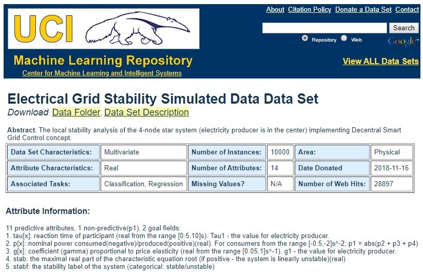
Dataset Particulars and Attribute Information
A Game-Plan for Predicting Stability in a Dynamic Process
So, the problem to be tackled is this: can we - given the data provided and what one would deem to be an acceptable degree of accuracy - predict the stability or instability of the electrical grid?
Time for some circumspective thought. There are a few things to ponder as we proceed through the interface with our toy question:
1. What are the Characteristics of the Dataset in General?
We have 10000 data points, 11 predictors and a choice of a numeric or categorical response variable. Normally, we’d have a time-stamped attribute to go along with these, but the author’s goal (see the DataSet Information at the website) is to simulate a dataset based on a prior academic paper. Having one must not have been appropriate to his needs.
With a legitimate date and time (and location!) you could tie in atmospheric conditions for potentially better predictions. And, you’d want to know a bit about the sensors that gathered the data. Can we track the sensor model and type along with the reading? Do some register inaccurately or drop data at random or in patterns? A skeptical eye towards data origin - on the whole, and by-column - is always a valuable trait to be embraced.
2. What are the Characteristics of the Dependent Variable?
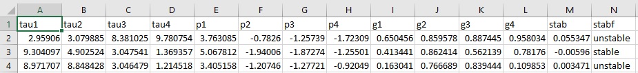
Since we’re predicting a Yes/No -or- Stable/Unstable outcome, this corresponds to the column stabf. We’ll want to check the splits between counts of stable and unstable values. You’d expect a dataset of real data - which this isn’t - to be largely populated with stable data. This would present some tasks regarding test/train stratification if that’s the case. Azure ML will allow us to get a feel for that distribution.
The column stab can be eliminated from the model. It’s the numeric version of the response variable. It’s unnecessary here because we’re only after a two-outcome categorical result - is the electrical grid stable or unstable?
3. What are the Characteristics of the Predictor Variables?
We’ll check out how predictors are distributed as we examine them in Azure. Please note the p1-p4 columns correspond to nominal power consumed, and p1 is not considered predictive. Why? note how it’s calculated: p1 = abs(p2 + p3 + p4).
You’re going to get a highly linear correlation between p1 and one or more of the other p-variables. more so if they’re all positive. So best to eliminate it, but we’ll take a look at the values for that and the remaining predictors as we continue in Azure ML.
4. What Predictive Modeling Methods and Evaluation Metrics Apply?
Classic binary-outcome Logistic Regression is an obvious choice to forecast a Stable/Unstable state for the electrical grid. And, with all the predictors numeric, we can also throw a Neural Network at the problem as well and see which one predicts better. Azure will give us:
A plot of the ROC curve.
The resultant area-under-the-curve (AUC) score, and
A slider control allowing us to see the effects on the False Positive / False Negative mix at different thresholds of probability for Stable and Unstable classifications.
And by the way, you’ll be able to compare both models simultaneously. That’s not an exhaustive list of what Azure can do for us when evaluating our models. But that’ll do for our example.
5. Beyond the Scoring: Factors Influencing Final Model Choice
Here we get to questions of model explainability. Neural Networks are notoriously difficult as a mechanism that explains why predictors give the results that they do, without diving into a discussion on a myriad of path weighting and back-propagation strategies with people whose eyes glaze over when you broach the subject. If you all have had better luck on that point than I, I’m all ears…
There’s no business context as to why you get a better predictive result from two or twenty layers of hidden nodes. Whereas with regression, you can coefficients and their signs as it relates to the context of the business or application. Even simple regression models can tell you a lot (wow, sunlight and moisture are positive contributors to forecasted crop growth. Who knew?).
If you have stakeholders offering you a lot of money for answers out of a model, odds are they’re going to want some backstory on what makes it tick. But not always. Sometimes only the answer is important to those that gain from it. But as our Data Science vocation and notions of ethically-built models mature (to be influenced in the U.S. by inevitable legislation, as with GDPR in the EU), methods - however accurate - that provide minimal backstory are going to be increasingly pushed to fringe applications. That’s the future, in my opinion. Open debates on that viewpoint are welcome. Let’s mold that future together…
Launching Azure ML Studio
It’s now nuts-and-bolts time. And I’m opening up the catnip now. With your account set up and access option chosen, you can sign into Azure ML Studio directly from the splash page noted in the prior post:

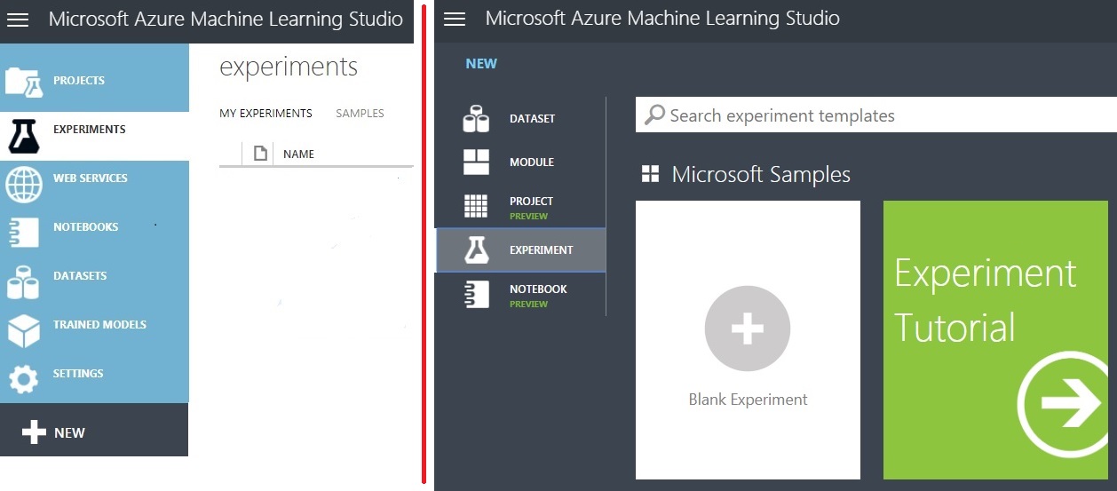
You should be thrown into a screen like the one we saw in our last post. From there:
Choose ‘Experiments’ and take the ‘+ New’ control. Select ‘Blank Experiment’.
Your First (Azure ML) Experiment
On the blank experiment screen, our blue object grouping section compresses to the left edge of the screen. Opening up to us in the new screen real-estate are the following:
A global section for commentary about the purpose of the experiment at the far right, as needed.
In the center, a drag-and-drop ‘canvas’ of steps that comprise the experiment, complete with connectors and connection points.
At the left, a list of ‘experiment items’ that will be subcomponents of the experiment. Each of these will have properties that we will administer to.
At the top, an experiment name. This can be overwritten; going forward I’ll be calling mine ‘Electrical Grid Predictive Trial’.
Once you change the title, click ‘Save’ at the bottom of the page.
![]()
Linking your Data to the Experiment
For now, hover your cursor over the Import Data item, underneath the Data Input and Output group. You’ll see from the hovertext that it allows you an option to load data manually, from the Web, or from several Azure sources. You can also use CSV files in Saved Datasets uploaded prior through the Datasets control (the icon of three data elements in blue). With our data easily accessible from UCI, we’ll just hit the URL directly.
Drag an ‘Import Data’ item over to the middle of the screen.
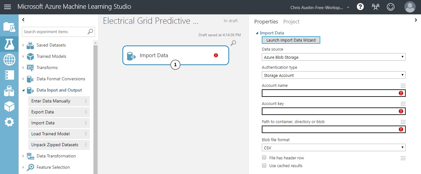
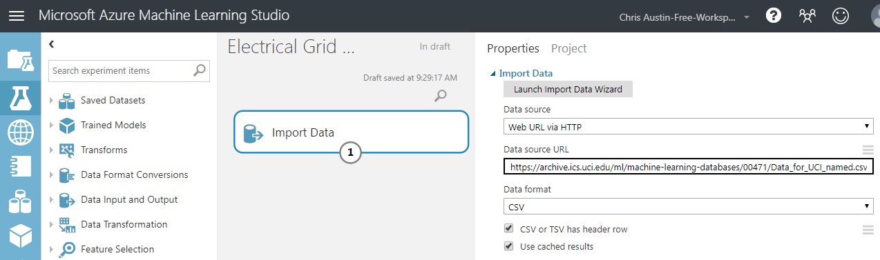
Not what you expected here? We can fix that and the errors shown on the screen. While you could just as easily progress through the Data Wizard, we’ll handle the process ourselves. For those following along at home, the following steps are necessary:
Switch ‘Data Source’ to ‘Web URL via HTTP’. - Your options change; the ‘Blob Storage’ choices seen on the screenshot disappear.
Add the URL seen in the screenshot below.
Set Data Format to CSV.
Check both the ‘Header Row’ box and the ‘Cached Results’ box. We saw a header row in our Excel excerpt earlier… And a helpful hint here - if you don’t choose ‘cached’, it’ll try to hit the URL every time you execute the experiment. If your dataset is static in nature, you’ll only need to pull it in once. I’d highly suggest checking that box unless you’re working with streaming or periodically-changing data and you’ve considered the ramifications of consistently longer run-times.
Click ‘Save’ at the bottom of the page.
Click ‘Run’ at the bottom of the page. When it’s finished, a green check-mark should appear in the ‘Import Data’ experimental item (see next section).
Seeing the data loaded into Azure
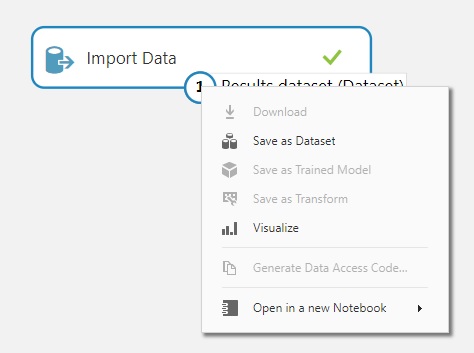
Now that you’ve run the experiment, let’s take a look at the ‘Results Dataset’ that was built. Notice the sole connector point - labeled ‘1’. Each experiment item has one or more connectors that either create (bottom) or expect (top) a restricted class of objects, whether they be data, models, or others as we’ll see going forward.
Click (right OR left) on the connection point and choose ‘Visualize’:
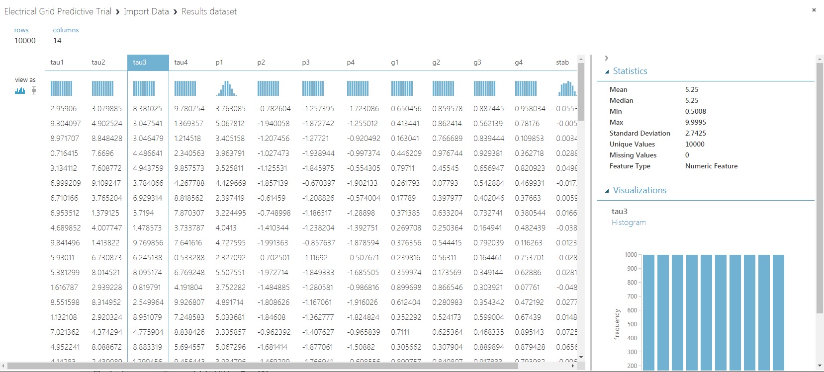
There are a couple of valuable items available to us here:
- An ability to look a predictor’s distribution using histograms and boxplots (Click on the histogram or boxplot under ‘view as’ to change that up).
- Some descriptive statistics for each predictor.
- A count of missing and unique values, and the perceived data type.
That’s plenty for now, I think. Don’t want to use all of the catnip at once…
What we’ll be tackling in the next post is the remainder of the data cleanup, some optional custom code to enhance our Exploratory Data Analysis, and the setup of our first of two models to predict electrical grid stability.
Further Information on the Subject:
A big thanks goes out to: Dua, D. and Graff, C. (2019). UCI Machine Learning Repository [http://archive.ics.uci.edu/ml]. Irvine, CA: University of California, School of Information and Computer Science.