Reticulate - Leveraging Python from R

Data Science Altitude for This Article: Camp One.

If you’re a Python developer that has been thrust into an R working environment or an R developer that would like to try out Python packages and methods in the comfort of an already-familiar RStudio IDE, then Reticulate is the package for you. Using rmarkdown, you’re able to knit R and Python code blocks into a unified whole and can refer to objects across the language barrier.

Graphing can not only be done through base plot() or ggplot() calls, but with a little effort we’ll show how to leverage your Python visualization skills using any of the matplotlib, seaborn, or (one of my favorites) bokeh packages.

Further, you have the opportunity to invoke an interactive Python session from within RStudio. How fun is that???

Let’s get to it…

```{r setup, warning = FALSE}
knitr::opts_chunk$set(echo = TRUE)
library(reticulate)
use_python("D:/Anaconda3") # Path to python3.exe
```

Our First Python Chunk

Our initial entry within the curly braces shows that this chunk should use the Python engine. The syntax in the remainder of the block should look rather familiar to Python developers and leverages the pandas package, home of Python’s Source and DataFrame data structure implementations. It’s part of the sciPy group of packages that all practicing open-source Data Scientists should be (or become…) familiar with.

You can find a copy of the flights.csv data file here, if interested. We’re taking a look at flights where the flight distance is less than 1800 miles. We’ll slim it down and look at just the carrier field and the arrival and departure differentials (both early and late) from the stated flight time, along with the distance flown. Nothing too strenuous, but enough to illustrate some of the reticulate’s functionality for cross-chunk data reference.

```{python}
import pandas as pd
flights = pd.read_csv("flights.csv")
flights = flights[flights['distance'] < 1800]
flights = flights[['carrier', 'dep_delay', 'arr_delay', 'distance']]
flights = flights.dropna()
print(flights.head())
```

##   carrier  dep_delay  arr_delay  distance
## 0      UA        2.0       11.0      1400
## 1      UA        4.0       20.0      1416
## 2      AA        2.0       33.0      1089
## 3      DL       -6.0      -25.0       762
## 4      UA       -4.0       12.0       719

Referencing Python structures in an R chunk

To reference Python variables in an R chunk, you have to preface them with ‘py$’:

```{r}
sprintf("%d of %d flights were delayed more than fifteen minutes.", 
        sum(py$flights$dep_delay > 15), length(py$flights$dep_delay))
```

## [1] "20221 of 118284 flights were delayed more than fifteen minutes."

Also, you can throw ggplot at them using they ‘py$’ reference, if your visualization skills are better with ggplot than the Python renderers:

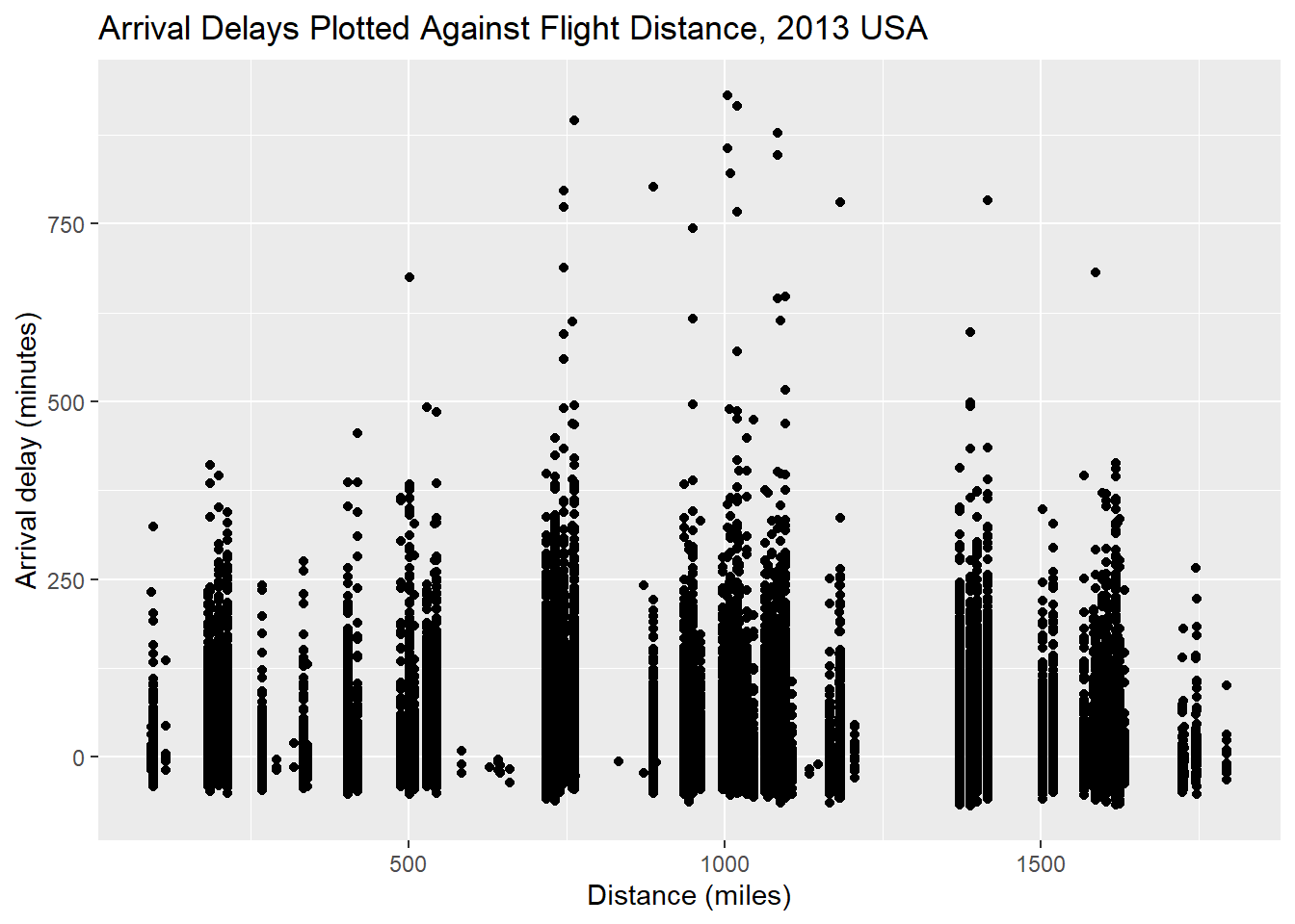
```{r}
library(ggplot2)
p <- ggplot(py$flights, aes(y = arr_delay, x = distance)) + geom_point()
p + labs(x = 'Distance (miles)', y = 'Arrival delay (minutes)', 
    title = 'Arrival Delays Plotted Against Flight Distance, 2013 USA')
```

Let’s take a look at what it takes in a Python chunk to refer to R data…

Referencing R structures in Python.

So, let’s reference a few variables from the python data that only exist in an R chunk. Below is the code to create the mean departure and arrival delays of the subset greater when zero. If you’re going to depart late or arrive late, what’s the average time without the influence of the times you were early?

```{r, collapse = TRUE}
meanDepDelay = mean(py$flights$dep_delay[py$flights$dep_delay > 0])
meanArrDelay = mean(py$flights$arr_delay[py$flights$arr_delay > 0])
```

You can do that in a Python block by using r.objectName:

```{python, collapse = TRUE}
print(r.meanDepDelay)
print(r.meanArrDelay)
```

## 34.518
## 36.381

Okay, so far so good. We can refer to R data in Python, and vice versa. But what if you’re wanting to roll the other direction - you’ve got r variables but are more comfortable throwing a Pythonic visualization out there? No problem, but there’s an extra step involved…

Using Python renderers within an rmarkdown block.

There’s one thing you need to do before trying a piece of code like this:

```{python, collapse = TRUE}
from math import cos, pi
import numpy as np
from mpl_toolkits.mplot3d import Axes3D
import matplotlib.pyplot as plt
from matplotlib import cm

xDomain = list(np.arange(-5.12, 5.12, .08))
yDomain = list(np.arange(-5.12, 5.12, .08))

X, Y = np.meshgrid(xDomain, yDomain)
z = [20 + x**2 + y**2 - (10*(cos(2*pi*x) + cos(2*pi*y))) for x in xDomain for y in yDomain]
Z = np.array(z).reshape(128,128)

fig = plt.figure(figsize = (12,10))
ax = fig.gca(projection='3d')
surf = ax.plot_surface(X, Y, Z, cmap=cm.RdYlGn, linewidth=1, antialiased=False)

ax.set_xlim(-5.12, 5.12)
ax.set_ylim(-5.12, 5.12)
ax.set_zlim(0, 80)
fig.colorbar(surf, aspect=30)

plt.title('Rastrigin Function in Two Dimensions: (Min at 0, Max at 80)\n 20 + x^2 + y^2 - 10*cos(2*pi*x) - 10*cos(2*pi*y)\n')
plt.show()
```

Looks good syntactically, but it will blow up on you.

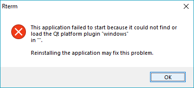
You’ll first need to set an environment variable for the PyQt cross-platform enablement package, bridging the C++ package Qt and Python. Again, Anaconda to the rescue:

import os 
os.environ['QT_QPA_PLATFORM_PLUGIN_PATH'] = 'D:\Anaconda3\Library\plugins\platforms'

Once you add in those lines before the plt.show() call, you’re good to go.

## (-5.12, 5.12)
## (-5.12, 5.12)
## (0, 80)
## <matplotlib.colorbar.Colorbar object at 0x000000001E1F3828>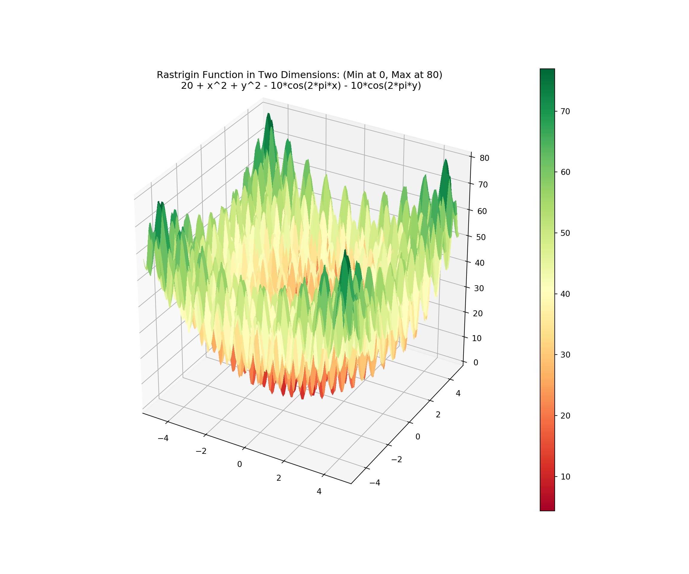

An Interactive Python Environment in the R Console

Running an interactive Python session in the R console is as simple as:

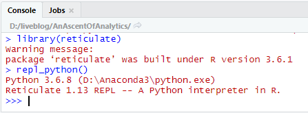
Note that it uses the version of python in our earlier use_python() call. From here, let’s try out some code that uses the Symbolic Python package sympy:

> repl_python()
Python 3.6.8 (D:\Anaconda3\python.exe)
Reticulate 1.13 REPL -- A Python interpreter in R.
>>> from sympy import Symbol, plot, Derivative, pprint, solve, Circle, Point
>>> from sympy.plotting import plot_parametric
>>> a,b,c,d,low,high = (-1.5, -12.3, 6, 500, -10, 10)
>>> x = Symbol('x')
>>> polyCubic = a*x**3 + b*x**2 + c*x + d
>>> 
>>> # The smallest y-value for positioning the axes of the plot doesn't necessarily 
>>> # have to happen at the low or high of the x ranges.
>>> yExtremes = (polyCubic.subs(x, high), polyCubic.subs(x, low))
>>> 
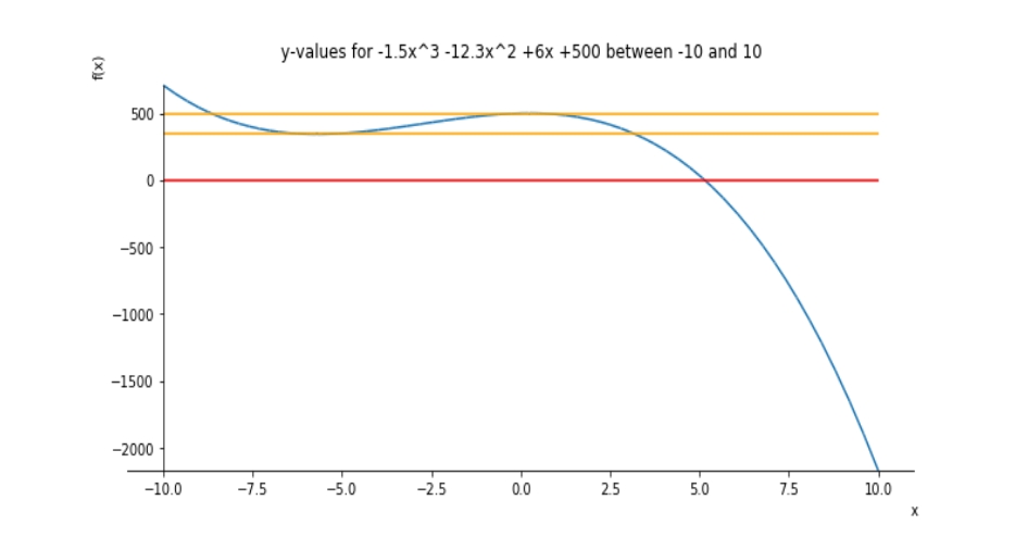
>>> p = plot(polyCubic, (x, low, high), axis_center = (low, min(yExtremes)),
...          title = "y-values for {0}x^3 {1:+}x^2 {2:+}x {3:+} between {4} and {5}".format(a,b,c,d,low,high),
...          show = False)

>>> # Determine derivative of equation and if roots are non-complex and can be plotted 
>>> dx =Derivative(polyCubic, x)
>>> dxSoln = dx.doit()        

>>> print("Derivative of Cubic equation is:")
Derivative of Cubic equation is:
>>> pprint(dxSoln, use_unicode = True)
       2             
- 4.5⋅x  - 24.6⋅x + 6
>>> 
>>> roots = solve(dxSoln)

>>> if isinstance(roots, complex):
...     print("Roots of the derivative have components in the complex plane (a + bi).")
... else:
...     point1 = polyCubic.subs(x, roots[0])
... point2 = polyCubic.subs(x, roots[1])          

>>> print("The real roots of the cubic derivative are x = {0:.3f} and x = {1:.3f}".format(roots[0], roots[1]))

The real roots of the cubic derivative are x = -5.701 and x = 0.234
>>> p2 = plot_parametric(x, 0, line_color = 'red', show = False)
>>> p.append(p2[0])
>>> p3 = plot_parametric(x, point1, line_color = 'orange', show = False)
>>> p.append(p3[0])
>>> p4 = plot_parametric(x, point2, line_color = 'orange', show = False)
>>> p.append(p4[0])
>>> p.show()

You should get something like this as an output:

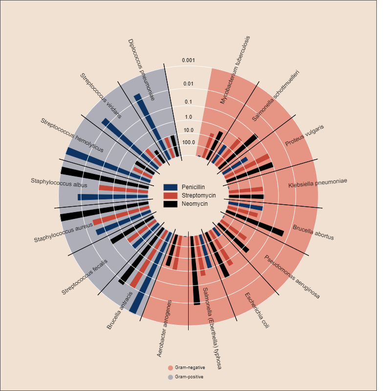
Let’s also try sourcing something from the command line. Here’s the output from a piece of python code from the bokeh gallery.

source_python('bokeh_source.py')

You should get something that looks like this in a separate HTML window:

Not much more to say, please take a look at all the documentation and enjoy !

Further Information on the Subject:

RMarkdown, explained. Kudos to Yihui Xie, J.J. Allaire, and Garrett Grolemund.

Reticluate pages: From RStudio and from Pablo Franco.